Data Ingestion
In Tensorflow the majority of users are most familiar with what is known as Feeding data. The Tensorflow feed mechanism allows users to inject data into any Tensor in their computational graph. Here is a simple example (original source).
Build And Profile A Model
with tf.Session():
  input = tf.placeholder(tf.float32)
  classifier = ...
  print(classifier.eval(feed_dict={input: my_python_preprocessing_fn()}))
We have built a simple model based on this paper that uses a feed dict to train. You can find the source code for our model here. There are two important aspects to this model.
First, you will see that we are using a feed_dict to run an interative optimization operation.
_, l = sess.run([train_op, loss], feed_dict={
    u_inputs: user_batch,
    i_inputs: item_batch,
    ratings_input: rating_batch
Second, note that the Batch_Dataset class is iterable, and that it has the __next__ function defined.
class Batch_Dataset(object):
    ...
    def __iter__(self):
        return self

    def __next__(self):
        self.iter += 1
        if self.iter > self.stop_iter:
            self.iter = 0
            raise StopIteration
        else:
            rand_indices = np.random.choice(range(len(self.ratings)), size=self.batch_size, replace=False)
            return (np.array(self.user_review_list[rand_indices]),
                    np.array(self.item_review_list[rand_indices]),
                    np.array(self.ratings[rand_indices]).reshape(self.batch_size, 1))
As defined our __next__ method will select a random subset from three numpy arrays, one containing user reviews of items, one containing reviews for an item by other users, and one containing the rating this user gave this item. It is important to note that this is text data that has already been cleaned and only needs to be converted to indices, then embeddings, in order to pass them through our network.
We use tensorflow to do the conversion by defining a HashTable and embeddings Variable.
table = tf.contrib.lookup.HashTable(
  tf.contrib.lookup.KeyValueTensorInitializer(keys, values), -1
)

word_embeddings = tf.get_variable(
    "word_embeddings",
    shape=[len(dictionary), emb_size]
)
We found that this model took 59.807 seconds to train to completion. Further, we found that the GPU reached at most 30% utilization.
+-----------------------------------------------------------------------------+
| Processes:                                                       GPU Memory |
|  GPU       PID   Type   Process name                             Usage      |
|=============================================================================|
|    0      2027      C   python                                     10941MiB |
+-----------------------------------------------------------------------------+
Sat Apr 21 22:34:11 2018
+-----------------------------------------------------------------------------+
| NVIDIA-SMI 390.30                 Driver Version: 390.30                    |
|-------------------------------+----------------------+----------------------+
| GPU  Name        Persistence-M| Bus-Id        Disp.A | Volatile Uncorr. ECC |
| Fan  Temp  Perf  Pwr:Usage/Cap|         Memory-Usage | GPU-Util  Compute M. |
|===============================+======================+======================|
|   0  Tesla K80           Off  | 00000000:00:1E.0 Off |                    0 |
| N/A   63C    P0    65W / 149W |  10954MiB / 11441MiB |     30%      Default |
+-------------------------------+----------------------+----------------------+
Getting The Most Out Of Tensorflow
For our case this may be sufficient. Waiting only one minute for a model to train is amazing compared to other models like AlphaGo which take 4 - 6 weeks even with all the resources available to DeepMind. According to the Tensorflow documentation here
If GPU utilization is not approaching 80-100%, then the input pipeline may be the bottleneck.
To see what may be holding us back from full gpu utilization we decided to run a check with the python profiler.
python -m cProfile -s tottime DeepCoNN\ -\ feed\ dict.py > profile.txt
Looking inside profile.txt we find the following.
   Ordered by: internal time

   ncalls  tottime  percall  cumtime  percall filename:lineno(function)
      825   17.388    0.021   17.388    0.021 {built-in method _pywrap_tensorflow_internal.TF_Run}
    58294   15.318    0.000   15.318    0.000 {built-in method numpy.core.multiarray.array}
    ...
As expected, our model spends the most time on some Tensorflow TF_Run which takes approximately 17.388 seconds. Interestingly, the next line shows us that the second most expensive method is a cast to Numpy arrays which almost takes just as long as the TF_Run calls. This begs the question, how do we remove this cast to numpy arrays?
Of course, Tensorflow has a built in api for Importing Data. They even have a performance guide, which we will use as a roadmap to change our model’s training process.
We can envision the problem with our model with the following image, taken from the Tensorflow performance guide link.
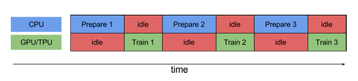
Our problem is actually twofold. First, our model is spending too much time waiting for python to break the dataset into random batches of Numpy arrays. Additionally, though less obvious, we then have to transfer that data from Python’s environment to the Tensorflow session. Both of these problems can be solved simultaneously using Tensorflow’s tf.data api. This api can ingest data from multiple file types like csv, text files, string inputs and even multiple files of those types. We will use tfrecords because they are described as the standard tensorflow format. For now we will assume you have your data in a binary *.tfrecords file of the proper format, but due to a lack of documentation, we will be making another, shorter, post on how to create these data files and work with the api.
Additionally, we will change our model to use the Estimator api to ingest data in order to handle variable, queue, and table initialization as well as removing the call to tf_run and feed_dict usage. You can find the final model here. Importantly, you will note that we have defined our model construction in a single function with model_fn(features, labels, mode). This model is fed data through the features parameter via an iterator built by the following function.
def get_dataset_iterator(loc, batch_size, max_len, pad_value):
    dataset = tf.data.TFRecordDataset(loc)
    dataset = dataset.prefetch(batch_size)
    dataset = dataset.map(parse_fn, num_parallel_calls=batch_size)
    dataset = dataset.map(split_fn, num_parallel_calls=batch_size)
    dataset = dataset.map(get_truncate_fn(max_len), num_parallel_calls=batch_size)
    dataset = dataset.padded_batch(batch_size, padded_shapes=([max_len], [max_len], [None]), padding_values=(pad_value, pad_value, 0.0))
    dataset = dataset.shuffle(26352)
    iterator = dataset.make_one_shot_iterator()
    return iterator
As we can see, this reads a tfrecords file from the location, prefetches a batch, parses the data, splits the data (we are working with strings), truncates strings that are too long, pads and batches strings that are too short, shuffles the full dataset (in our case we know there are 26352 data points) then returns an iterator that traverses each data point. For now we will assume some familiarity with reading tfrecord files, but in another post we will have more documentation on doing so.
By using tfrecords and the tf.data api our model is able to train in 30.879 seconds. Again, think in percentages of improvement rather than absolute terms, our 30 second improvement is actually 50% less time to train the model. This could be a 4 - 6 week training time turning into a 2 - 3 week training time. Looking at our GPU utilization, we actually got as high as 61% at some points! Approaching the 80% utilization the Tensorflow documentation specifies as an approximate heuristic.
+-----------------------------------------------------------------------------+
| Processes:                                                       GPU Memory |
|  GPU       PID   Type   Process name                             Usage      |
|=============================================================================|
|    0      2101      C   python                                     10941MiB |
+-----------------------------------------------------------------------------+
Sat Apr 21 22:35:18 2018
+-----------------------------------------------------------------------------+
| NVIDIA-SMI 390.30                 Driver Version: 390.30                    |
|-------------------------------+----------------------+----------------------+
| GPU  Name        Persistence-M| Bus-Id        Disp.A | Volatile Uncorr. ECC |
| Fan  Temp  Perf  Pwr:Usage/Cap|         Memory-Usage | GPU-Util  Compute M. |
|===============================+======================+======================|
|   0  Tesla K80           Off  | 00000000:00:1E.0 Off |                    0 |
| N/A   66C    P0   106W / 149W |  10954MiB / 11441MiB |     61%      Default |
+-------------------------------+----------------------+----------------------+
Finally looking at the python profile we can obviously see that our cast to numpy is gone, and the most time consuming process was TF_Run which took about 24 seconds because it now includes all of our data ingestion as well as model training.
   Ordered by: internal time

   ncalls  tottime  percall  cumtime  percall filename:lineno(function)
      851   24.341    0.029   24.341    0.029 {built-in method _pywrap_tensorflow_internal.TF_Run}
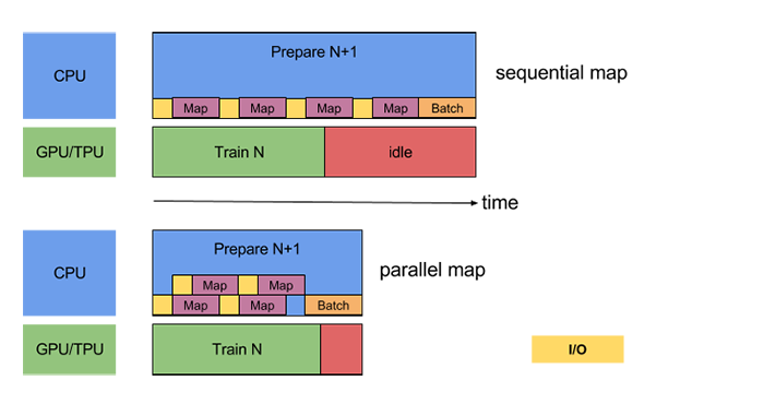
What we can imagine having happening now is that the Tensorflow api is able to read and preprocess data prior to our model requesting more data to train on. Rather than all the time spent idle as above, our model training now looks like the bottom diagram in the following image during each iteration.
In conclusion, inference and model training times have opportunity for vast improvement using simple, well known tools and concepts. Simply using the recommended input format, parallelizing data collection and preprocessing improved our training time by 50% which in long-running models is significant.